
Crash Course on PyTorch and Autograd
I’ve been recently working with Variational Autoencoders (VAE) and I’ve stumbled upon an interesting paper titled “The Riemannian geometry of deep generative models” by Shao et al.
One of the main concepts of working with high-dimensional data is the manifold hypothesis: we suppose that the observed data is concentrated around a low-dimensional manifold. It is for instance reasonable to surmise that cat pictures are actually a microscopic subset of all possible pictures. (To be fair, whether or not the subspace in which they live is indeed a manifold remains to be proven, but it is not the subject of this post).

Left: projection along the manifold, right: observed data; in the first case, projecting along the manifold makes the data linearly separable; in the second case, it doesn’t.
Shao et al. provide an algorithm to compute geodesic paths between points on the generated manifold without the need to find the underlying equation of the manifold. This paragraph from Wikipedia explains the specificity of geodesics quite well:
In general, geodesics are not the same as “shortest curves” between two points, though the two concepts are closely related. The difference is that geodesics are only locally the shortest distance between points, and are parameterized with “constant speed”. Going the “long way round” on a great circle between two points on a sphere is a geodesic but not the shortest path between the points. The map \( t \mapsto t^2 \) from the unit interval on the real number line to itself gives the shortest path between 0 and 1, but is not a geodesic because the velocity of the corresponding motion of a point is not constant. Geodesics are commonly seen in the study of Riemannian geometry and more generally metric geometry. In general relativity, geodesics in spacetime describe the motion of point particles under the influence of gravity alone. In particular, the path taken by a falling rock, an orbiting satellite, or the shape of a planetary orbit are all geodesics in curved spacetime.
I might be wrong here, so please do correct me if that is the case, but, in theory, if your generative model is really good, your latent space should be homeomorphic to the manifold and a geodesic on the manifold should be obtained by a straight line in the latent space. In practice, that will almost never happen, so you might need to adjust the straight line, which is what this algorithm does.
For more details on the math involved, I will let the reader refer to the paper. In the aforementioned algorithm, one needs to compute the following gradients for \( i \in \{1, \dots, T-1\}\):
\[ \nabla_{z_i} E = -\frac{1}{\delta_T} \, J_g^T(z_i) \, \big(g(z_{i+1}) - 2 \, g(z_i) + g(z_{i-1})\big) \]where \( T \) is the number of steps, \( \delta_T \coloneqq 1 / T\), \( (z_0, \dots, z_T) \) is the discrete geodesic path (so each \( z_i \) is a vector in the latent space), and \( g \) is the decoder of the generative network.
I’ve always tried to avoid dealing with gradient computing in PyTorch, but here I haven’t had much of a choice. I figured I might as well record it for future use. Who knows, maybe it’ll help you too.
Backward() in PyTorch
I strongly advise you to read the suggested resources at the end of this post, but I’ll try to explain as clearly as possible the basics of automatic differentiation and how I implemented the stuff.
First, let me ask you a question: when you call loss.backward() in a neural network, do you know what actually happens?
Don’t worry, neither did I before yesterday. I had a vague idea but that was all.
When PyTorch applies operations on tensors initialized with requires_grad set to True, thanks to a library called autograd (docs here), it keeps track of all operations it does under the hood in what is called a dynamic computational graph. That way, when you call the backward function, it just has to parse the graph in the reverse direction to compute the gradients: that is called automatic differentiation.
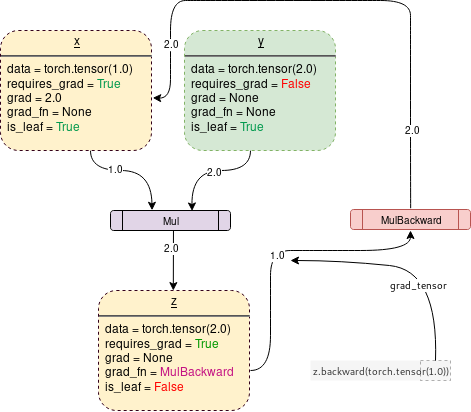
DCG with requires_grad = True
The code corresponding to this image could look like this:
x = torch.tensor(1.0, requires_grad=True)
y = torch.tensor(2.0)
z = x * y
z.backward()
print(x.grad)  # tensor(2.)
The backward() call populates x.grad with the gradient of z with respect to x. In that case, x.grad will be equal to tensor(2.) since \(
\del{z}{x} = y = 2 \).
Great, so we just have to do the same to get the Jacobian right?
# given a tensor u with requires_grad=True:
v = g(u)
v.backward()
print(u.grad)  # RuntimeError: grad can be implicitly created only for scalar outputs
Well… Not quite. For efficiency purposes, autograd never actually computes the Jacobian: it always computes vector-Jacobian products so it doesn’t have to store the whole Jacobian in memory.
To be more accurate, given a function \[ f : \bb{R}^m \to \bb{R}^n \]
autograd only computes vector-Jacobian products of the following form:
where \( v \in \bb{R}^n \) is a vector of the output space and \[ \del{f}{x} = \begin{bmatrix} \del{f_1}{x_1} & \cdots & \del{f_1}{x_m} \\ \vdots & \ddots & \vdots \\ \del{f_n}{x_1} & \cdots & \del{f_n}{x_m} \end{bmatrix} \]
Backpropagation w.r.t. a Scalar Output
Let me show you a basic example of how it works with a scalar output:
Let \( \quad x = \begin{bmatrix} 2 \\ 3 \end{bmatrix}\), \( \quad A = \begin{bmatrix} 3 & 1 \\ 1 & 0 \\ 0 & -2 \end{bmatrix}\), \( \quad y = Ax = \begin{bmatrix} 9 \\ 2 \\ -6 \end{bmatrix}\),
and \( \quad \mcal{L} = y \cdot \begin{bmatrix} 1 \\ -1 \\ 1 \end{bmatrix} = 9 - 2 - 6 = 1\).
By the chain rule, we have \[ \del{\mcal{L}}{x} = \del{\mcal{L}}{y} \del{y}{x} = \begin{bmatrix} 1 & -1 & 1 \end{bmatrix} \begin{bmatrix} 3 & 1 \\ 1 & 0 \\ 0 & -2 \end{bmatrix} = \begin{bmatrix} 2 & -1 \end{bmatrix}\]
However, what actually goes on, if I understand well, is this:
\[ \del{\mcal{L}}{x_1} = \del{\mcal{L}}{y} \del{y}{x_1} = \begin{bmatrix} 1 & -1 & 1 \end{bmatrix} \begin{bmatrix} 3 \\ 1 \\ 0 \end{bmatrix} = 2\] \[ \del{\mcal{L}}{x_2} = \del{\mcal{L}}{y} \del{y}{x_2} = \begin{bmatrix} 1 & -1 & 1 \end{bmatrix} \begin{bmatrix} 1 \\ 0 \\ -2 \end{bmatrix} = -1\]
This is better because you do not have to load the whole Jacobian \( \del{y}{x} \) in memory at once, and you do not lose efficiency because all those computations can be parellelized.
The drawback is that you can not directy access the Jacobian, but since the primary purpose of backpropagation is enabling gradient descent, in most use cases the Jacobian is not needed, only the gradient w.r.t. the loss is.
Now I’ll unveil a somewhat hidden truth about backward: it always computes a vector-Jacobian product, even if the output is scalar. Hence, when you call backward(), what really happens is that backward(torch.tensor(1.0)) is called instead. Since you simply multiply the Jacobian (which is here of the same size as the input vector \(
x \)) by the scalar 1, it’s transparent. Now, the error message RuntimeError: grad can be implicitly created only for scalar outputs is clearer: when the output is scalar, backward assumes the vector by which to multiply the Jacobian is torch.tensor(1.).
So now, let’s say we want to backpropagate w.r.t. a vector output: how do we proceed?
Backpropagation w.r.t. a Vector Output
Let us reuse the previous example, but let us say that we now simply want to compute the Jacobian \( \del{y}{x} \), which here is equal to \( A \).
Short answer: you can’t.
Long answer: you can, but it’s very rarely needed. Even for my initial purposes, if you look back at the expression of \( \nabla_{z_i} E \), you can see that it is actually a sum of (transposed) vector-Jacobian products, so I do not actually need the whole Jacobian.
Case #1: Only vector-Jacobian products are needed
For example, let’s say you want to compute the vector-Jacobian products \[ v^T \, \del{y}{x} \] where \( v \in \bb{R}^3 \).
You simply have to define \[ \mcal{L} = y^T v \] and backpropagate from \( \mcal{L} \).
If you look closely, it’s actually exactly the same as the previous case with \( v = \begin{bmatrix} 1 \\ -1 \\ 1 \end{bmatrix} \)!
Here is a very neat interpretation of the vector term in vector-Jacobian product: it can be seen as the gradient of a loss with respect to the vector output!
Indeed, in the previous case, \[ v = \left( \del{\mcal{L}}{y} \right)^T \]
I personally find that interpretation much easier to work with than simply seeing it as needing an arbitrary vector product to compute a Jacobian.
Case #2: The whole Jacobian is needed
In that case, a way to get the Jacobian is to compute all of its vector-Jacobian products with the basis vectors which I will write \( (e_i)_{i \in \{1, \dots, n\} } \). Indeed, for \( i \in \{1, \dots, n\} \), we have \[ e_i \, \del{y}{x} = A_i\] where \( A_i \) is the i-th row of \( A \).
All that is left is to concatenate all the rows to retrieve the matrix. Make sure that you can’t solve your problem another way though, as the Jacobian tends to be quite big in deep learning settings.
Back to the Initial Problem
Let us now see how to compute our initial gradients. For simplicity’s sake, I’ll remove the multiplicative factor: \[ \nabla_{z_i} E = J_g^T(z_i) \, \big(g(z_{i+1}) - 2 \, g(z_i) + g(z_{i-1})\big) \]
# given a tensor z with requires_grad=True:
x = g(z)
for i in range(1, g.shape[0] - 1):
    x[i].backward(-2 * x[i].detach(), retain_graph=True)  # (1)
    x[i].backward(x[i - 1].detach(), retain_graph=True)  # (2)
    x[i].backward(x[i + 1].detach(), retain_graph=True)  # (3)
print(z.grad)  # what we want!
- At call (1),
backwardpopulatesz.grad[i]with the vector \( J_g^T(z_i) \, \big(- 2 \, g(z_i)\big) \) (to be exact, its transposed value) sincex[i]depends only onz[i];
Another property of backward is that it always accumulates gradients by summing them;
- Therefore, at call (2),
backwardadds toz.grad[i]the value \( J_g^T(z_i) \, g(z_{i-1}) \); - At call (3),
backwardadds toz.grad[i]the value \( J_g^T(z_i) \, g(z_{i+1}) \);
At that point, we have: \[ \mathtt{z.grad[i]} = J_g^T(z_i) \, \big(g(z_{i+1}) - 2 \, g(z_i) + g(z_{i-1})\big) \]
- Remark #1: we call
detach()on the inputs ofbackwardbecause we only need the values of the tensors. Not callingdetach()might yield errors due to interference with the DCG; - Remark #2: we set the argument
retain_graphto True because otherwise,backwardclears the DCG. It is meant to free up space but in that specific case we need to keep the DCG since we backpropagate several times;
To conclude, here is the whole algorithm:
# given a tensor z of size (T, n) with requires_grad=True and z.grad=None:
while z.grad is None or (
    torch.sum(torch.norm(z.grad, dim=1) ** 2) > eps / (T ** 2)
):
    z.grad = None
    x = g(z)
    for i in range(1, T - 1):
        x[i].backward(-2 * x[i].detach(), retain_graph=True)
        x[i].backward(x[i - 1].detach(), retain_graph=True)
        x[i].backward(x[i + 1].detach(), retain_graph=True)
    with torch.no_grad():
        for i in range(1, T - 1):
            z[i] = z[i] + alpha * T * z.grad[i]
- Remark #3: we reset
z.gradtoNoneat the start of each loop; - Remark #4: we deactivate gradient computation as we update the geodesic path to avoid useless computations.
We’ve come to the end of the problem, at long last. Or have we?
Next Level: a Trick for Computing Jacobian-Vector Products
In the paper by Shao et al., they suggest to compute the following Jacobian-vector products instead: \[ \eta_i = J_h\big(g(z_i)\big) \, \big(g(z_{i+1}) - 2 \, g(z_i) + g(z_{i-1})\big) \] where \( h \) is the corresponding encoder to \( g \) such that \( h(g(z)) = z \).
The attentive reader will have noticed that the Jacobian is not transposed in that expression, which is quite troublesome since we seemingly have no way to transpose it in the automatic differentiation process. Fortunately, math nerds will always find a trick to make stuff work, and in that case this trick works like a charm.
Let us define the operator \[ \mathrm{vjp}(f)(v, x) \coloneqq v^T \del{f}{x}(x) \] where \( \mrm{vjp} \) stands for vector-Jacobian product.
Now let us treat \( x \) as a constant and let us consider the function \( \varphi : \bb{R}^n \to \bb{R}^m \) defined by: \[ \varphi(v) \coloneqq [\mrm{vjp}(f)(v, x)]^T = \left[ \del{f}{x}(x) \right]^T v \]
We can see that \( \varphi \) is a linear function of \( v \). Its Jacobian w.r.t. \( v \) is therefore constant w.r.t. \( v \) and verifies \[ J_\varphi = \left[ \del{f}{x}(x) \right]^T \]
Now let us reapply the \( \mrm{vjp} \) operator to \( \varphi \):
\[ \begin{aligned} \mrm{vjp}(\varphi)(u,v) &= u^T \del{\varphi}{v}(v) \\ &= u^T \left[\del{f}{x}(x) \right]^T \\ &= \left[ \left[ \del{f}{x}(x) \right] u \right]^T \end{aligned}\]Henceforth, by transposing the result, we have: \[ [ \mrm{vjp}(\varphi)(u,v) ]^T = \left[ \del{f}{x}(x) \right] u \] which is exactly what we want.
In practice, how do we compute this with PyTorch? First, I will let the reader refer to this PyTorch Forums thread which provides a Google Colab notebook implementing a possible solution which involves the method autograd.grad documented here.
If we keep the same code as earlier, here is one way to implement the trick:
v = torch.zeros_like(
    z[0], requires_grad=True
)  # requires_grad=True is required for jvps, but it will remain None
vjps = torch.zeros_like(x)
jvps = torch.zeros_like(z)
z_pred = h(x)
for i in range(1, T - 1):
    vjps[i] += torch.autograd.grad(
        z_pred[i], x, v, create_graph=True,
    )[0][i]
    jvps[i] += torch.autograd.grad(
        vjps[i], v, -2 * x[i], create_graph=True,
    )[0][i]
    jvps[i] += torch.autograd.grad(
        vjps[i], v, x[i - 1], create_graph=True,
    )[0][i]
    jvps[i] += torch.autograd.grad(
        vjps[i], v, x[i + 1], create_graph=True,
    )[0][i]
As magical as it looks, jvps will contain exactly what we want, i.e.
Parting Words
All in all, I’m glad I went through all that trouble of gathering all the information I could find and writing this post: I now feel much more confident in both manipulating vector dervatives and Jacobians, and in implementing it in a neural network model in PyTorch. As Einstein said,
If you can’t explain it simply, you don’t understand it well enough.
I believe I explained the concepts involved as simply as one could reasonably expect. At the very least, I sure do understand automatic differentiation better than before, so I’d call the mission a success.
By all means, feel free to tell me if there is a mistake somewhere or if it was helpful to you too!
Recommended Reading
- Towards Data Science - PyTorch Autograd - Understanding the heart of PyTorch’s magic
- PyTorch Forums - Computing vector-Jacobian and Jacobian-vector product efficiently
- Deep yearning - A new trick for calculating Jacobian vector products
- PyTorch Docs - Automatic differentiation package - torch.autograd
- Saihimial Allu - How exactly does torch.autograd.backward( ) work?